Using Multiple Time Dimensions for Data Quality Monitoring
A popular feature in Lariat is the ability to recognize multiple timestamp fields in raw data, and allow users to express Indicators using these timestamps, as well as toggle the time axis of their charts.
In this post we will dig into why it might be useful to maintain multiple timestamps on event data, and some interesting ways of working with those timestamps to assess data quality and pipeline health.
Generally speaking a data pipeline will have at least two notions of time to contend with when dealing with raw event data.
Event Time: Where the row of data being processed represents a real-world event taking place, such as a button being clicked or a mobile device pinging a network, event time is the timestamp of that event occurring. This timestamp is generally determined and attached to the data payload by the source system.
Ingest Time: This is the time at which the processing system actually ingests that row of data. It may be quite close to the event time, if the system is operating in near-real-time, or it may be some time later if either side of the pipe is delayed. This timestamp is attached downstream of the source system.
In addition a pipeline may decide to attach more timestamps to the data row as it flows through the system, perhaps as a way of “checkpointing” the time a row is handled by a node in the DAG.
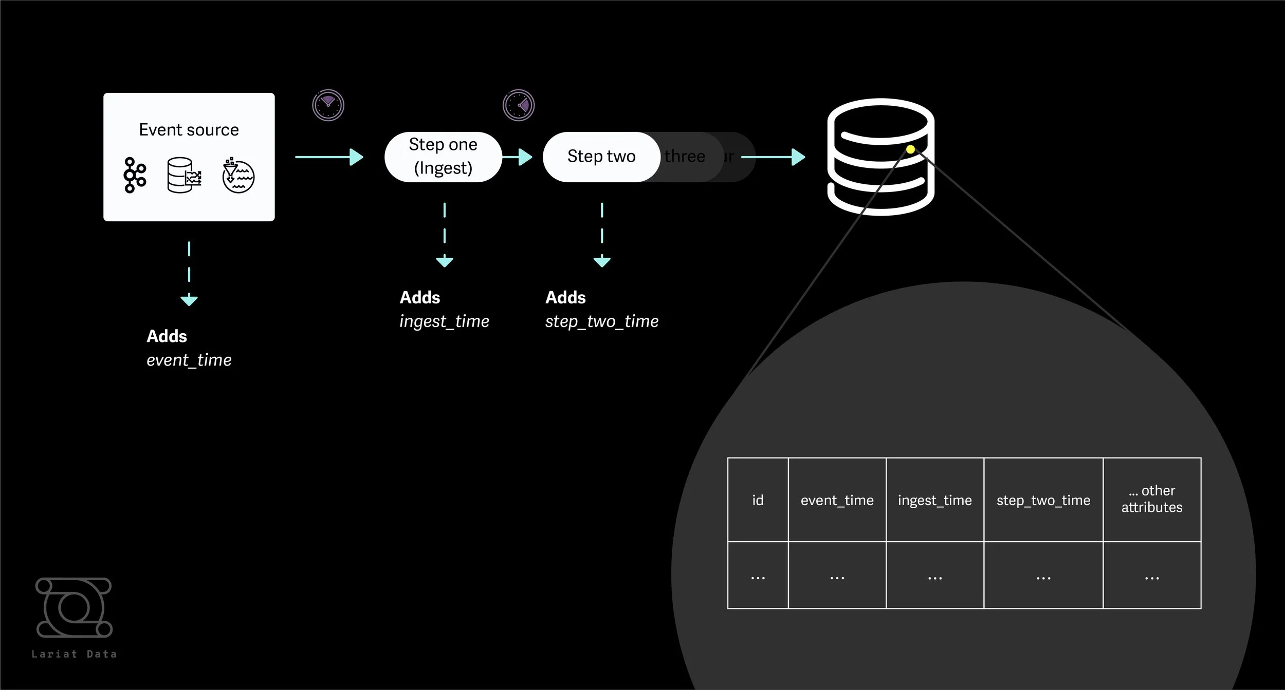
Materializing these timestamp fields into the data warehouse can be useful for debugging problems at the row or datum-level as well for the dataset in aggregate. Let’s walk through a few examples below.
Measuring Data Freshness
(The below examples use Snowflake’s TIMESTAMPDIFF function, but similar functions will exist in other SQL engines for computing the difference between timestamps)
Consider a table in a data warehouse that stores both event_time and ingest_time as row-level attributes.
To compute the delay between event and ingest for a single row, one might run a query such as:
SELECT TIMESTAMPDIFF(‘second’, ingest_time,event_time) FROM my_timestamped_table WHERE id = $1Delays can also be rolled up into an aggregated measure of data delay. For example,
SELECT AVG(TIMESTAMPDIFF(‘second’, ingest_time, event_time))
    AS avg_delay
    FROM my_timestamped_table
And if this aggregated measure is too coarse-grained or skewed by outliers, you can also place delays into discrete buckets with a quick case statement.
SELECT COUNT(*), (CASE WHEN TIMESTAMPDIFF('second', ingest_time, event_time) <= 60 THEN 'less than 1 minute'
    WHEN TIMESTAMPDIFF('second', ingest_time, event_time) <= 3600 THEN 'less than 1 hour'
    WHEN TIMESTAMPDIFF('second', ingest_time, event_time) <= 14400 THEN '1-4h'
    ELSE '4h+' END
) AS freshness FROM my_timestamped_table GROUP BY freshness
Result:
| COUNT(*) | freshness |
|---|---|
| 1,009,662 | less than 1 minute |
| 17,641,009 | less than 1 hour |
| 3,916,420 | 1-4h |
| 7803 | 4h+ |
The above query is using the CASE syntax to assign a freshness bucket to each row, depending on the timestamp delay between ingest and event times. The result is a handy summarization. In this case, it shows that although there are some outlier rows ingested more than 4 hours after the event time, most rows are processed in less than an hour.
The choice of ingest_time and event_time here express a common case for many data models, but in truth any two timestamp markers may be used to measure and communicate freshness.
Troubleshooting Using Rolling Time Windows
As tables grow and pipeline code evolves, many teams start to prioritise data quality in recent windows of time rather than measurements that scan the entirety of rows in the table. When data is loaded incrementally, a rolling time window allows you to collect measurements that are scoped just to new rows of data.
For example, the following Snowflake query would measure the count of rows in just the last hour of data by event time:
SELECT COUNT(*) from my_timestamped_table WHERE event_time >= (CURRENT_TIMESTAMP - INTERVAL '1hour') AND event_time <= CURRENT_TIMESTAMPMeasured over several advancing time windows this would produce a graph like below

Consider a case such as the below, where row count by event_time was consistent but abruptly stopped reporting a few hours ago.
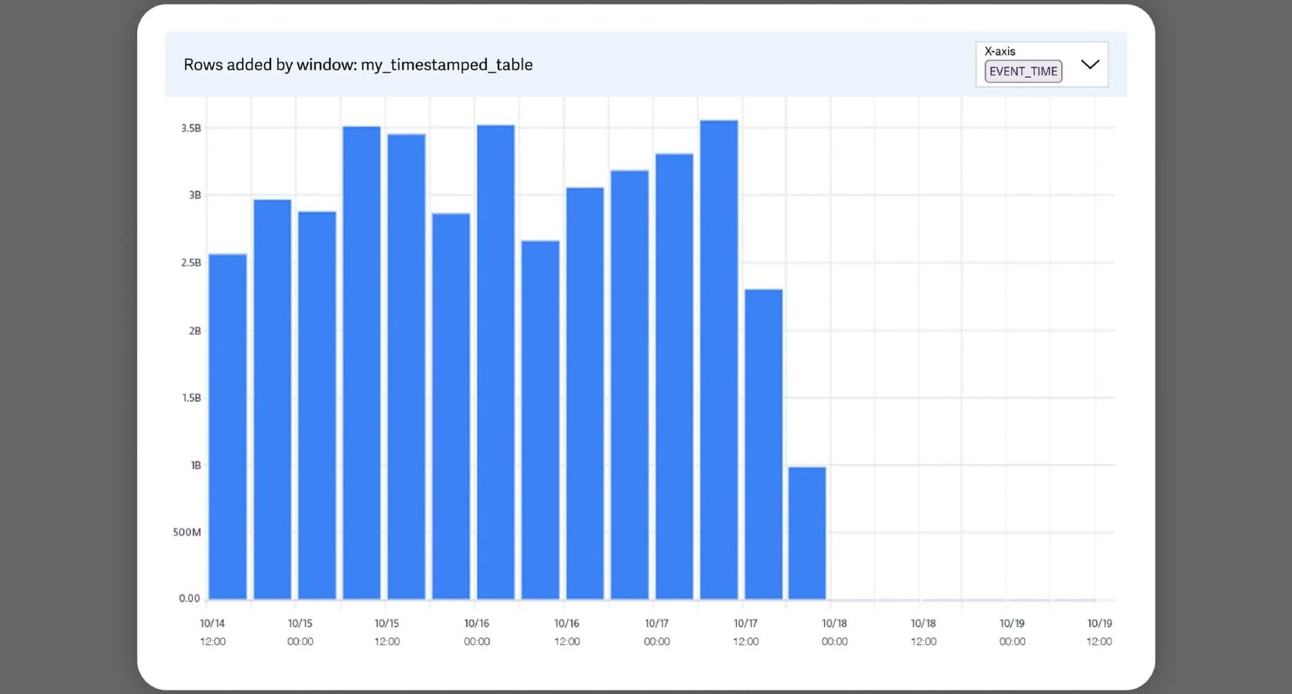
Engineers can quickly pinpoint whether the problem lies in the source system or in the ingestion phase, by graphing row count with ingest_time on the X-axis.

In fact our earlier freshness measurement, which created discrete freshness buckets, can further underline this conclusion. By looking at the delta of ingested_time and event_time for rolling ingested_time windows, it becomes clear that recent ingestion runs have been processing events > 4 hours old.

Since data freshness is now explicit, and granular, delayed and out-of-order data are immediately obvious, as is the severity of the delay. Importantly, the pipeline operator has not spent valuable time debugging the ingestion process and can instead focus efforts on understanding why source data is delayed.
This capability can extend to phases downstream of ingestion as well. As long as each phase adds a time checkpoint, any delay between pipeline phases becomes clear to the operator.
Operational Views for Different Stakeholders
Widening your dataset to include multiple timestamps also allows you to be flexible to the variety of reporting requirements within your organization.
Most business stakeholders will expect reports by Event Time e.g. daily sales reported by the day a user completed a purchase, as opposed to the day that purchase data was made available to the merchant’s backend. An ops team may obsess over the delay between event_time and a notional delivery_time, to enforce a guarantee of same-day delivery. Thanks to the truncation options provided by SQL Engines (e.g DATE_TRUNC in Snowflake), producing day-over-day or week-over-week reports on each of these time dimensions is also achievable.
By accommodating multiple timestamps in your tables, you can allow each of these stakeholders to extract a report catered to their line-of-business and avoid them having to work with data on a misaligned time axis. This is especially important as pipelines increase in complexity and ownership of pipeline phases becomes split between teams. Issues can be quickly triaged and pinpointed to a pipeline phase, and remediation work can be assigned to the right team.
Coda: Leveraging Indexes and Clustering
Range queries in the WHERE clause such as timestamp >= (CURRENT_TIMESTAMP - INTERVAL '1hour') AND timestamp <= CURRENT_TIMESTAMP can become expensive at larger data volumes, and it is often prudent to build an index on the timestamp field in question. With several timestamp fields, and thus several indexes, you can expect insertion time for rows to be moderately affected as a trade-off.
Some engines such as Snowflake also provide the option of a Clustering Key, which is an instruction to the storage engine to co-locate rows on disk that share the same key. Timestamps have theoretically unbounded cardinality, and you may not see performance improvements by clustering on a timestamp with second or sub-second granularity. If your storage engine allows it, consider using a truncation expression on the timestamp column as the Clustering Key, rather than the timestamp column directly. A tip from Snowflake’s documentation on clustering:
If a fact table has a TIMESTAMP column c_timestamp containing many discrete values (many more than the number of micro-partitions in the table), then a clustering key could be defined on the column by casting the values to dates instead of timestamps (e.g. to_date(c_timestamp)). This would reduce the cardinality to the total number of days, which typically produces much better pruning results.
We hope that reading this has given you some food for thought on how collecting additional timestamps within your data pipelines can enhance your data quality efforts. A nice thing about this approach is that it can work incrementally, and it is a good idea to begin with timestamping the most latency-sensitive portions of your pipeline first. In our experience, the payoff in identifying and troubleshooting data freshness issues, and creating stakeholder-specific views, can quickly offset the initial engineering investment in materializing additional timestamps.
If you haven’t tried Lariat out, you can be up and running with our Continuous Data Quality monitoring platform in minutes! Check us out here.


